Plotting Substitutions
Refer to this page to learn about how to plot single base substitutions (SBS) using the plotSBS function. Included below is the function and a list of valid parameter values. There are also examples of each SBS graph with a quick description for interpreting it.
plotSBS Function
The plotSBS function provides a standard approach for displaying mutational signatures and mutational patterns of single base substitutions. Depending on the specified parameters, the function can generate a number of distinct representations of signatures/patterns.
plotSBS(matrix_path, output_path, project, plot_type, percentage=False, custom_text_upper=None, custom_text_middle=None, custom_text_bottom=None)
or if you are running the R-wrapper package, any "False" must be changed to FALSE, "True" changed to "TRUE", and "None" changed to "NULL."
- matrix_path -> (String) The path to your matrix (generated by SigProfilerMatrixGenerator)
- output_path -> (String) The path to where the output will be saved
- project -> (String) The output file will have this value postfixed in the name.
- plot type -> (String) The plot type to be generated. Valid inputs include {"6", "24", "96", "384", and "1536"}.
- percentage -> (Boolean) True for a normalized percentile plot and False for a numerical plot. This parameter has a default value of False.
- custom_text_upper, custom_text_middle, custom_text_bottom -> (List of Strings) Provide a list of strings for adding a custom text to the upper right-hand corner of the plot. Ideally, there should be one string per sample. Extra strings will not be plotted. The three parameters allow for three rows of custom text (upper, middle, lower).
Supported SigProfiler Matrices include: 6, 24, 96, 384, and 1536.
plotSBS Examples
The following examples were generated in a python environment where sigProfilerPlotting was imported as sigPlt.
$ python3
>>import sigProfilerPlotting as sigPlt
From within a R session, you will import the library as follows:
$ R
>> library("reticulate")
>> use_python("path_to_your_python3")
>> py_config()
>> library("SigProfilerPlottingR")
The matrices below are used to generate the example plots. You can download and run the commands to generate the example plots. - SBS-6 - SBS-24 - SBS-96 - SBS-384 - SBS-1536
Plot SBS-6 Numerical
From within a Python session:
sigPlt.plotSBS(matrix_path_SBS + "SBS6.all", output_path, project_name, "6", percentage=False)
From within a R session:
>> plotSBS(matrix_path_SBS + "SBS6.all", output_path, project_name, "6", percentage=FALSE)
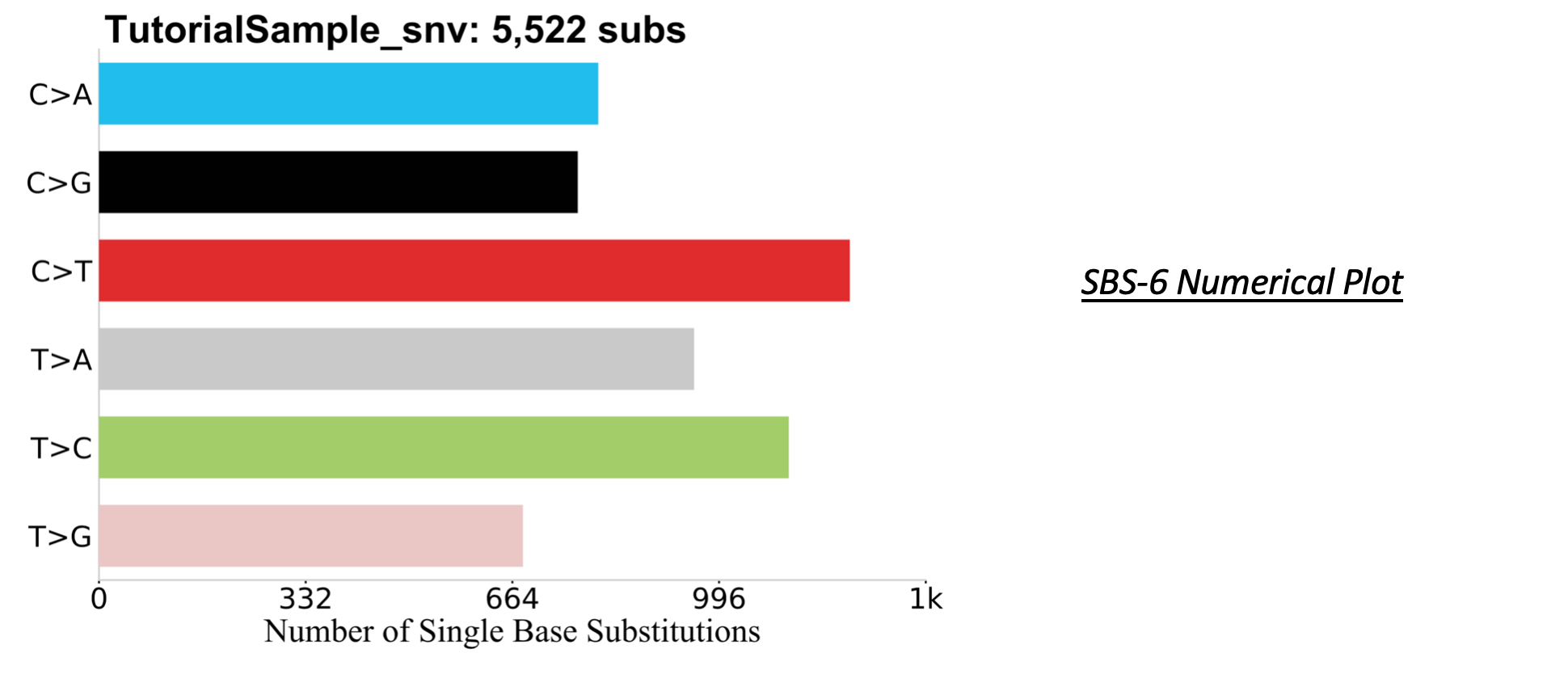 The Single Base Substitution-6 (SBS-6) numerical plot has the six different mutation categories on the y-axis and the number of each mutation on the x-axis. The sample name and total number of substitutions are provided at the top of the plot.
Plot SBS-6 Percentile
From within a Python session:
sigPlt.plotSBS(matrix_path_to_SBS_file + "SBS6.all", output_path, "BRCA_example", "6", percentage=True)
From within a R session:
plotSBS(matrix_path_to_SBS_file + "SBS6.all", output_path, "BRCA_example", "6", percentage=TRUE)
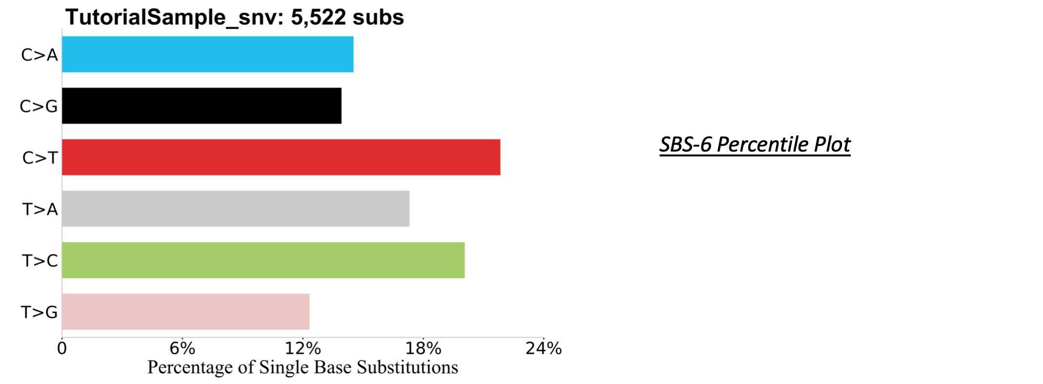 The Single Base Substitution-6 (SBS-6) percentile plot includes the six different mutation categories on the y-axis and the normalized percentages of each mutation on the x-axis.
Plot SBS-24
From within a Python session:
sigPlt.plotSBS(matrix_path_SBS + "SBS24.all", output_path,"BRCA_example", "24",False)
From within a R session:
plotSBS(matrix_path_SBS + "SBS24.all", output_path,"BRCA_example", "24",FALSE)
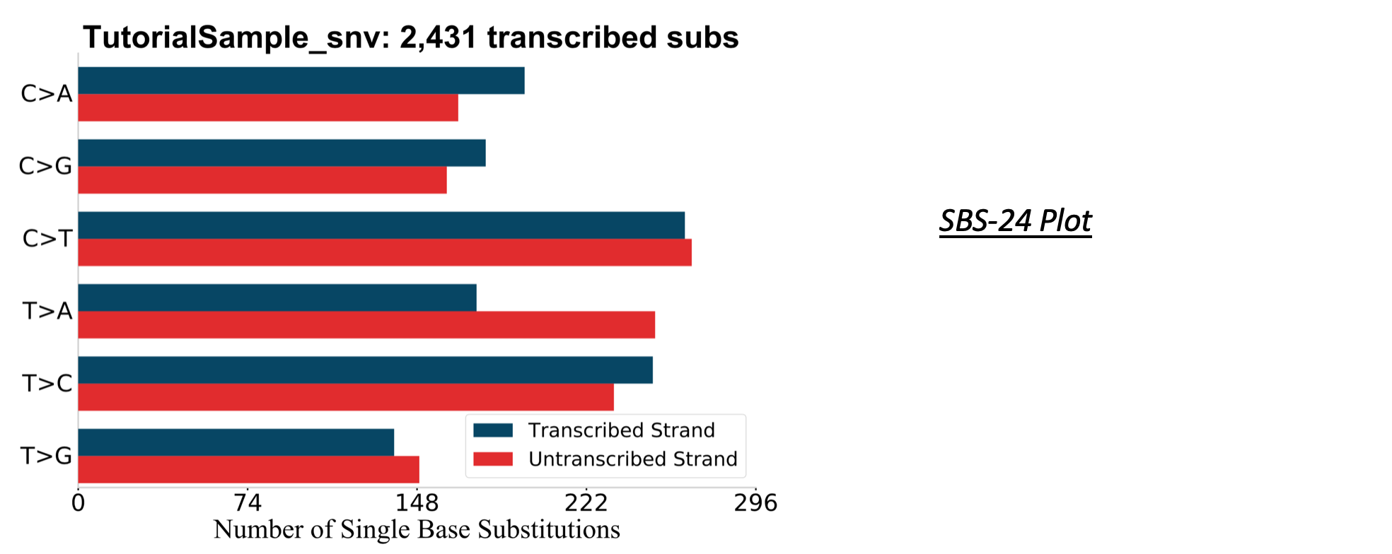 The Single Base Substitution-24 (SBS-24) numerical plot includes the six different mutation categories on the y-axis , and the number of mutations that occurred on the transcribed and untranscribed strands on the x-axis (does not plot bidirectional and nontranscribed TSB categories).
Plot SBS-96
From within a Python session:
sigPlt.plotSBS(matrix_path_SBS + "SBS96.all", output_path,"BRCA_example", "96",False)
From within a R session:
plotSBS(matrix_path_SBS + "SBS96.all", output_path,"BRCA_example", "96",FALSE)
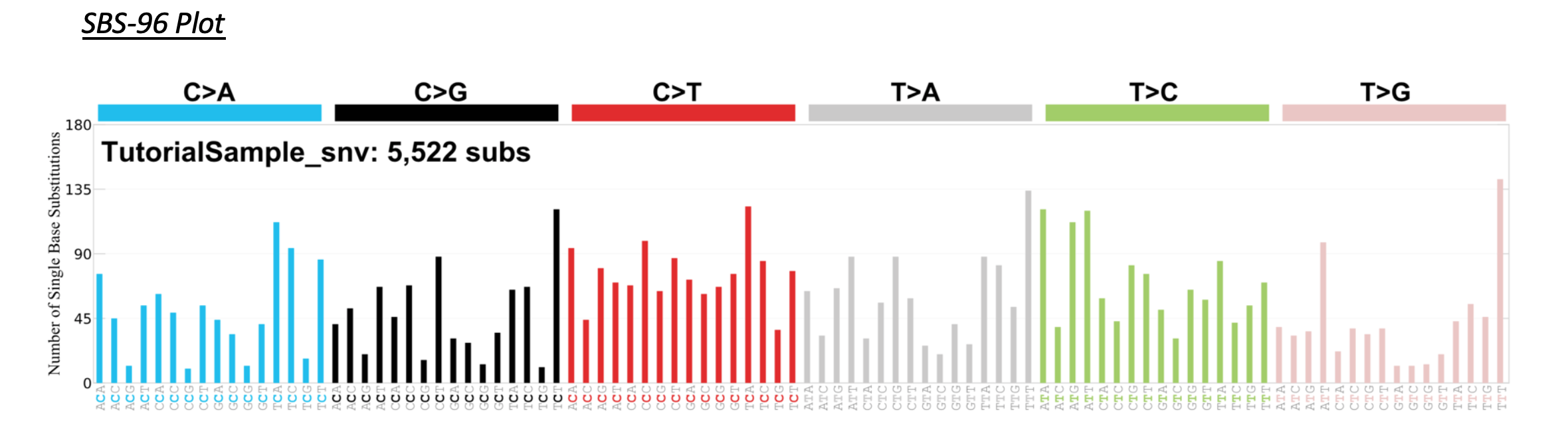 The Single Base Substitution-96 (SBS-96) numerical plot graphs the trinucleotide contexts of each mutation. Along the x-axis are the six main categories that represent the different mutations (C>A, C>G,...,T>G). Each of these six categories has an additional 16 categories to represent the combinations of bases that can prefix and postfix the mutation (ie. ACA, ACC, ACG, ACT, CCA,..., TCT). The y-axis presents the number of each mutation.
Plot SBS-384
From within a Python session:
sigPlt.plotSBS(matrix_path_SBS + "SBS384.all", output_path,"BRCA_example", "384",False)
From within a R session:
plotSBS(matrix_path_SBS + "SBS384.all", output_path,"BRCA_example", "384", FALSE)
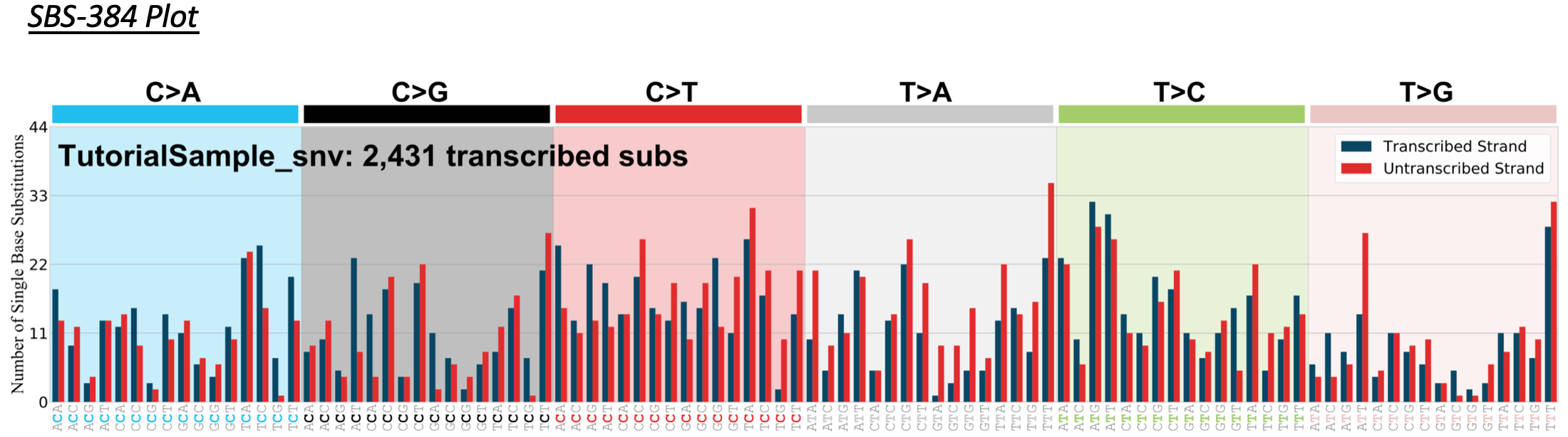 The Single Base Substitution-384 (SBS-384) numerical plot graphs the trinucleotide contexts of each mutation. Along the x-axis are the six main categories that represent the different mutations (C>A, C>G,...,T>G). Each of these six categories has an additional 16 categories to represent the combinations of bases that can prefix and postfix the mutation (ie. ACA, ACC, ACG, ACT, CCA,..., TCT). Additionally, the mutation is categorized depending whether it was located on the transcribed or untranscribed strand. The y-axis is the number of such mutations that occurred.
Plot SBS-1536
From within a Python session:
sigPlt.plotSBS(matrix_path_SBS + "SBS1536.all", output_path,"BRCA_example", "1536",False)
From within a R session:
plotSBS(matrix_path_SBS + "SBS1536.all", output_path,"BRCA_example", "1536",FALSE)
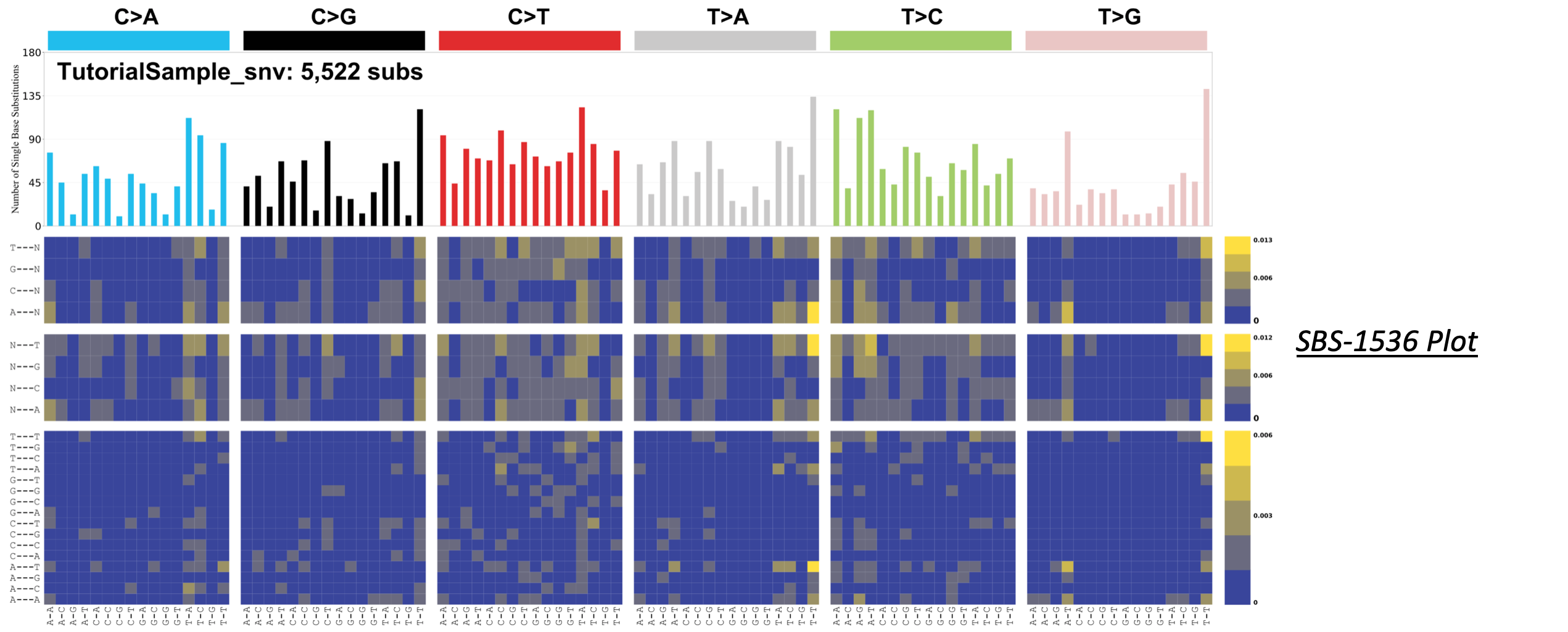
The Single Base Substitution-1536 (SBS-1536) numerical plot graphs the trinucleotide contexts of each mutations. Along the top on the x-axis are the six main categories that represent the different mutations (C>A, C>G,...,T>G). Directly below these categories are a set of bar graphs that have the number of each mutation. Also, beneath the bar graphs are heat maps of the pentanucleotide contexts. The probability is normalized to the maximum pentanucleotide count.